Metaballs and WebGL
I’m back to learning graphics! A lot of interesting simulation and rendering work takes place on the GPU, and I didn’t have much experience doing that, so I figured I’d try to get metaballs rendering on the GPU. This time, instead of using the marching squares algorithm, we’ll leverage the GPU to compute every pixel in parallel!
In this post, I’m going to walk through the steps of getting metaballs rendering with WebGL. Each step will have a separate codepen you can play with, and a list of suggestions for things to try in order to understand the concepts. To get the most out of this post, work through the challenges in the comments at the top of each codepen.
To focus on what’s happening at a low level, we’ll be using WebGL directly, and not a high-level abstraction library like the excellent THREE.js.
The OpenGL programmable pipeline
Let’s look at a simplified version of the OpenGL programmable pipeline. This is the pipeline of steps that brings you from 3D geometry to pixels on the screen using the GPU.
If you’ve never seen this before, don’t worry. As you walk through the code examples below, you might want to refer back to this diagram.

Shaders in OpenGL/WebGL are programs written in a C-like language called GLSL.
Vertex shaders operate on vertex property data, one vertex at a time. This
vertex property data is specified as attributes. Attributes might include
things like the position of the vertex in 3D space, texture coordinates, or
vertex normals. Vertex shaders set the magic gl_Position variable, which
GL interprets as the position in 3D space of the vertex. Vertex shaders are also
responsible for setting varying variables, which are consumed in the
fragment shader.
After positions are set in the vertex shader, the positions of the vertices are
passed to geometry assembly, which decides how the vertices are connected
into edges and faces based on the argument to gl.drawElements or
gl.drawArrays. For instance, if you specify gl.GL_LINE_STRIP, then
geometry assembly will connect every adjacent pair of vertices by edges, and
give you no faces. If you instead specify gl.GL_TRIANGLE_STRIP, then every
contiguous triple of vertices will be formed into a triangle.
Next, the geometry goes through rasterization, where each face or line is turned into pixels that fit the grid of the output framebuffer. Information about each one of these pixels, including the interpolated values of the varying variables, is then passed to the fragment shader.
Fragment shaders output the color for a specific pixel to the framebuffer.
As input, they have access to any varying variables specified in the vertex
shader, and a few magic variables like gl_FragCoord. As output, fragment
shaders set the magic gl_FragColor variable to specify the final color of the
pixel.
Uniform variables are available in both the vertex shader and fragment shader, and hold the same value regardless of which vertex or fragment the shader is operating on.
Aside: programmable vs fixed pipeline
While learning about OpenGL, and specifically WebGL, I was getting confused a lot about all the steps that were taking place. When I looked at how pixels got to the screen from geometry using shaders, I kept asking questions like: “Where is the camera set up?“, “How are coordinates converted from the world coordinate system to the view coordinate system?“, “How do I set the scene’s lighting”?
The answer to all of these questions is, in the world of the programmable pipeline, all of these things are up to you. There’s no default concept of a camera, or model coordinates, or lighting, or Phong shading. It’s all up to you.
This is in contrast to older GPUs and older versions of OpenGL which used a fixed pipeline, where you would set all those things directly and it would figure out how to convert from world coordinates to camera view coordinates and light the scene for you.
You can read a lot more about it in this excellent article: The End of Fixed-Function Pipelines (and How to Move On).
Step 1. Running a fragment shader for every pixel on the screen
To be able to run arbitrary computation to determine the color of every pixel in our canvas, we need to get a fragment shader running for every pixel on the screen.
First, we set up geometry that covers the whole screen. The fragment shader only runs for pixels inside geometry being drawn, and also only for pixels that have x and y coordinates in between -1 and 1 (these coordinates are called normalized device coordinates). These coordinates will be stretched by GL to fit the viewport (i.e. these numbers always vary between -1 and 1, regardless of canvas size and aspect ratio).
To cover the screen perfectly, we’ll set up two triangles like so:
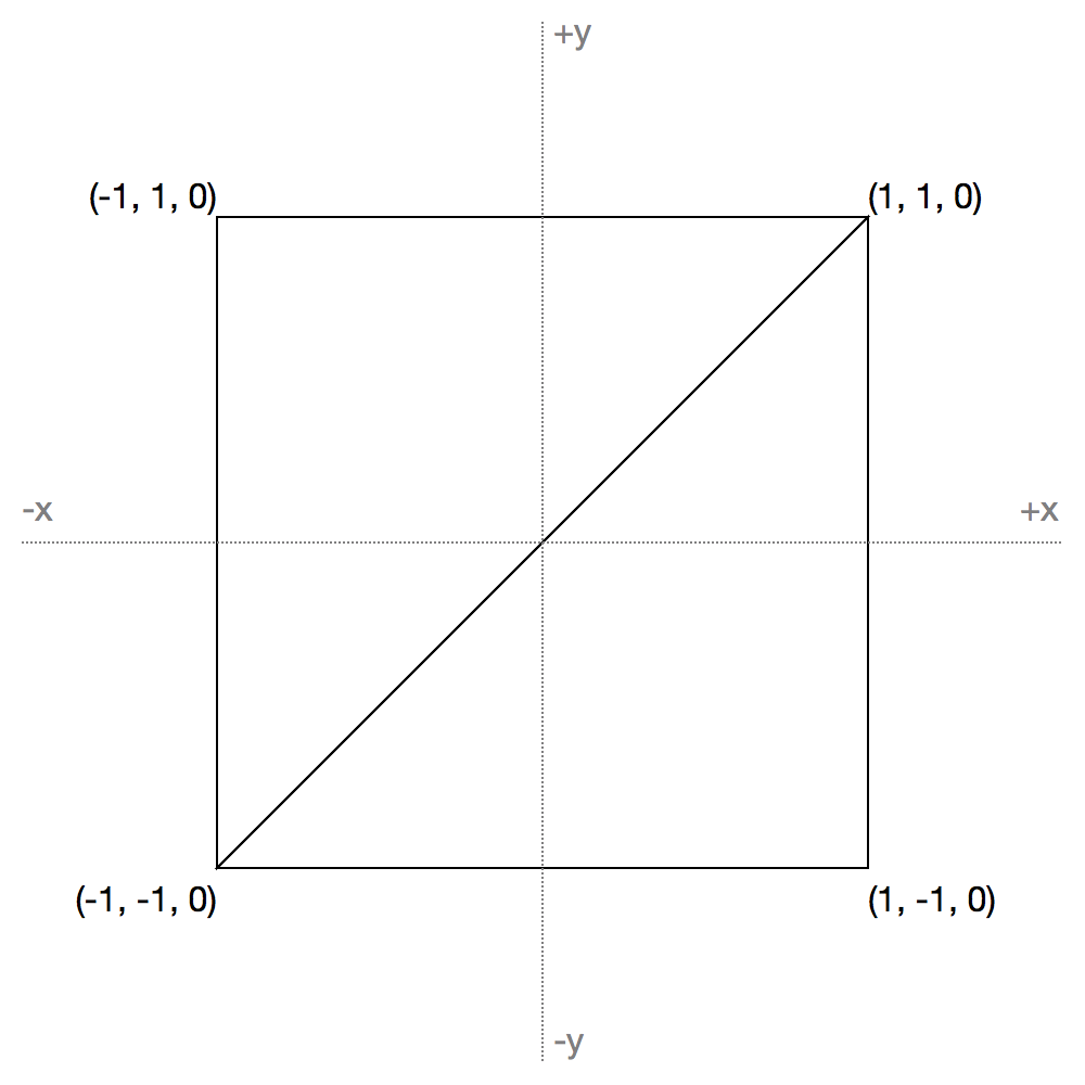
See the Pen WebGL Metaballs Part 1 by Jamie Wong (@jlfwong) on CodePen.
Click “Edit on codepen” and explore the code for it – I commented the code just for you! In a comment at the top, I’ve included some things to try out to deepen your understanding of the code.
Step 2. Doing something different for each pixel
Running a computation for each pixel isn’t helpful if you do the same thing for
each pixel. To have different information for each pixel, we could either set
useful varying variables in our vertex shader, or we can use gl_FragCoord.
We’ll opt for the second option here.
See the Pen WebGL Metaballs Part 2 by Jamie Wong (@jlfwong) on CodePen.
The only thing changed between steps 1 and 2 is the fragment shader. Here’s the new fragment shader code:
void main(){
    gl_FragColor = vec4(gl_FragCoord.x/500.0,
                        gl_FragCoord.y/400.0,
                        0.0, 1.0);
}
Just as last time, click on “Edit on codepen”, and read through the challenges at the top.
Step 3. Moving data from CPU to GPU
In step 2, we managed to make each pixel do something different, but the only information available there was the coordinates of the pixel. If we’re trying to render metaballs, we need to get the information about the radius and positions of the metaballs into the fragment shader somehow.
There are a few ways of making an array of data available in a fragment shader.
First option: uniform arrays
Uniforms in GLSL can be integers or floats, can be scalars or vectors, and can
be arrays or not. We can set them CPU-side using
gl.uniform[1234][fi][v].
If we set a uniform via gl.uniform3fv, then inside the shader, we can access
it with a declaration like so:
uniform vec3 metaballs[12]; // The size has to be a compile time constant
This has the benefit of being easy to use, but has a major downside of having a low cap on the size of the array. GL implementations have a limit on the number of uniform vectors available in fragment shaders. You can find that limit like so:
gl.getParameter(gl.MAX_FRAGMENT_UNIFORM_VECTORS)
Which is 512 on my machine. That means the following compiles:
uniform highp float vals[512];
But the following gives me ERROR: too many uniforms when I try to compile the
shader:
uniform highp float vals[513];
This limit is for the whole shader, not per-variable, so the following also doesn’t compile:
uniform highp float vals[256];
uniform highp float vals2[257];
512 is probably good enough for our purposes since we aren’t going to have hundreds of metaballs, but wouldn’t be good enough for transferring information about thousands of particles in a particle simulation.
Second option: 2D textures
Second option: 2D textures. Textures can be constructed on the CPU via
gl.createTexture, gl.bindTexture, and be populated with
gl.texImage2D. To make it available in the fragment shader, a uniform
sampler2D can be used.
The benefit of using textures is that you can transfer a lot more data. The limits on texture size seem a bit fuzzy, but WebGL will at least let you allocate a texture up to 1xMAX pixels, where MAX can be found with:
gl.getParameter(gl.MAX_TEXTURE_SIZE)
Which is 16384 on my machine. In practice, you probably won’t be able to use a texture at 16384x16384, but regardless you end up with a lot more data to play with than 512 uniforms vectors. In practice I’ve had no issues with 1024x1024 textures.
Another benefit is that if you’re clever, you can run simulations entirely on the GPU by “ping ponging” between textures: flipping which one is input and which one is output to move forward a timestep in your simulation without needing to transfer any of the simulation state between CPU and GPU memory. But that’s a topic for another day.
The downside is that they’re kind of awkward to use: instead of indexing
directly into an array, you need to convert your array index into a number in
the range [0, 1], correctly configure the texture’s filtering algorithms
to be nearest neighbour to avoid dealing with bizarre interpolation between your
array elements, and if you want support for real floating point numbers, your
users’ browsers and devices have to support the OES_texture_float
extension.
Third option: compile the array data into the shader
The benefit of GLSL code being compiled at JavaScript runtime is that you can generate GLSL code from JavaScript and compile the result. This means you could generate GLSL function calls as needed, one per element in your array.
This is one of the techniques used in the awesome WebGL Path Tracing demo.
Implementation with uniform arrays
For our purposes, since we’re not transferring massive amounts of data, we’ll go with the easiest option of using uniform arrays. To the codepen!
See the Pen WebGL Metaballs Part 3 by Jamie Wong (@jlfwong) on CodePen.
Most of the change needed to get to this step is in the fragment shader and in new sections at the bottom labelled “simulation setup”, and “uniform setup”.
If you want to send a vec3 array from CPU to GPU, you’ll need a
Float32Array with 3 times the number of elements as the vec3 array.
Here’s a snippet of the code that deals with this conversion and sending it to the GPU.
var dataToSendToGPU = new Float32Array(3 * NUM_METABALLS);
for (var i = 0; i < NUM_METABALLS; i++) {
    var baseIndex = 3 * i;
    var mb = metaballs[i];
    dataToSendToGPU[baseIndex + 0] = mb.x;
    dataToSendToGPU[baseIndex + 1] = mb.y;
    dataToSendToGPU[baseIndex + 2] = mb.r;
}
gl.uniform3fv(metaballsHandle, dataToSendToGPU);
Step 4. Animation and blobbiness
That’s pretty much it for the tricky WebGL bits! The last bit is applying the
same math as in the first part of the Metaballs and marching squares post
inside the fragment shader, and then sticking the whole thing in a timer loop
using requestAnimationFrame, along with a bit of logic to make the balls
move around and bounce off the walls.
See the Pen WebGL Metaballs Part 4 by Jamie Wong (@jlfwong) on CodePen.
Resources
Thanks for reading! Here are some of the resources that I read to help me understand OpenGL, GPUs, and WebGL:
- Tiny Renderer: Learn how OpenGL works by making your own!
- How a GPU Works: This helped me understand what’s happening inside a GPU at a lower level, and reason about performance. For instance, this helped me better understand why branching is so expensive on the GPU.
- Unleash Your Inner Supercomputer: Your Guide to GPGPU with WebGL: A fairly thorough but occasionally confusing explanation behind using WebGL for computation as opposed to rendering. Reading through the code was instructive.
- lightgl.js: A lightweight, simpler, but lower level abstraction over
WebGL than THREE.js. All of the code for it is documented thoroughly using
docco. Reading through the code for parts like
GL.Shaderhelped me understand WebGL’s APIs better. - An intro to modern OpenGL. Chapter 1: The Graphics Pipeline: A much more thorough explanation of the graphics pipeline, with much better diagrams than this post.
- OpenGL ES Shading Language Reference: A concise overview/cheatsheet of GLSL.