Ray Marching and Signed Distance Functions

I’ve always been fascinated by demoscenes: short, real-time generated audiovisual demos, usually in very, very small executables. This one, by an artist named “reptile”, comes from a 4KB compiled executable. No external assets (images, sound clips, etc.) are used – it’s all in that 4KB.

To get a intuitive grip on how small 4KB is, a 1080p video that this produces is 40MB, or ~10,000 times larger than the executable that produces it. Keep in mind that the executable also contains the code to generate the music.

One of the techniques used in many demo scenes is called ray marching. This algorithm, used in combination with a special kind of function called “signed distance functions”, can create some pretty damn cool things in real time.

Signed Distance Functions

Signed distance functions, or SDFs for short, when passed the coordinates of a point in space, return the shortest distance between that point and some surface. The sign of the return value indicates whether the point is inside that surface or outside (hence signed distance function). Let’s look at an example.

Consider a sphere centered at the origin. Points inside the sphere will have a distance from the origin less than the radius, points on the sphere will have distance equal to the radius, and points outside the sphere will have distances greater than the radius.

So our first SDF, for a sphere centered at the origin with radius 1, looks like this:

$$ f(x, y, z) = \sqrt{x^2 + y^2 + z^2} - 1 $$

Let’s try some points:

$$ \begin{aligned} f(1, 0, 0) &= 0 \\ f(0, 0, 0.5) &= -0.5 \\ f(0, 3, 0) &= 2 \end{aligned} $$

Great, $ (1, 0, 0) $ is on the surface, $ (0, 0, 0.5) $ is inside the surface, with the closest point on the surface 0.5 units away, and $ (0, 3, 0) $ is outside the surface with the closest point on the surface 2 units away.

When we’re working in GLSL shader code, formulas like this will be vectorized.
Using the Euclidean norm, the above SDF looks like this:

$$ f(\vec{p}) = ||\vec{p}|| - 1 $$

Which, in GLSL, translates to this:

float sphereSDF(vec3 p) {
    return length(p) - 1.0;
}

For a bunch of other handy SDFs, check out Modeling with Distance Functions.

The Raymarching Algorithm

Once we have something modeled as an SDF, how do we render it? This is where the ray marching algorithm comes in!

Just as in raytracing, we select a position for the camera, put a grid in front of it, send rays from the camera through each point in the grid, with each grid point corresponding to a pixel in the output image.

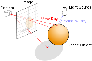
The difference comes in how the scene is defined, which in turn changes our options for finding the intersection between the view ray and the scene.

In raytracing, the scene is typically defined in terms of explicit geometry: triangles, spheres, etc. To find the intersection between the view ray and the scene, we do a series of geometric intersection tests: where does this ray intersect with this triangle, if at all? What about this one? What about this sphere?

Aside: For a tutorial on ray tracing, check out scratchapixel.com. If you’ve never seen ray tracing before, the rest of this article might be a bit tricky.

In raymarching, the entire scene is defined in terms of a signed distance function. To find the intersection between the view ray and the scene, we start at the camera, and move a point along the view ray, bit by bit. At each step, we ask “Is this point inside the scene surface?”, or alternately phrased, “Does the SDF evaluate to a negative number at this point?“. If it does, we’re done! We hit something. If it’s not, we keep going up to some maximum number of steps along the ray.

We could just step along a very small increment of the view ray every time, but we can do much better than this (both in terms of speed and in terms of accuracy) using “sphere tracing”. Instead of taking a tiny step, we take the maximum step we know is safe without going through the surface: we step by the distance to the surface, which the SDF provides us!

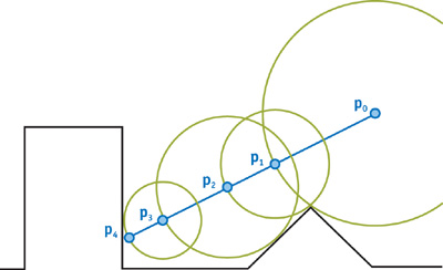
In this diagram, $ p_0 $ is the camera. The blue line lies along the ray direction cast from the camera through the view plane. The first step taken is quite large: it steps by the shortest distance to the surface. Since the point on the surface closest to $ p_0 $ doesn’t lie along the view ray, we keep stepping until we eventually get to the surface, at $ p_4 $.

Implemented in GLSL, this ray marching algorithm looks like this:

float depth = start;
for (int i = 0; i < MAX_MARCHING_STEPS; i++) {
    float dist = sceneSDF(eye + depth * viewRayDirection);
    if (dist < EPSILON) {
        // We're inside the scene surface!
        return depth;
    }
    // Move along the view ray
    depth += dist;

    if (depth >= end) {
        // Gone too far; give up
        return end;
    }
}
return end;

Combining that with a bit of code to select the view ray direction appropriately, the sphere SDF, and making any part of the surface that gets hit red, we end up with this:

Voila, we have a sphere! (Trust me, it’s a sphere, it just has no shading yet.)

For all of the example code, I’m using http://shadertoy.com/. Shadertoy is a tool that lets you prototype shaders without needing to write any OpenGL/WebGL boilerplate. You don’t even write a vertex shader – you just write a fragment shader and watch it go.

The code is commented, so you should go check it out and experiment with it. At the top of the shader code for each part, I’ve left some challenges for you to try to test your understanding. To get to the code, hover over the image above, and click on the title.

Surface Normals and Lighting

Most lighting models in computer graphics use some concept of surface normals to calculate what color a material should be at a given point on the surface. When surfaces are defined by explicit geometry, like polygons, the normals are usually specified for each vertex, and the normal at any given point on a face can be found by interpolating the surrounding vertex normals.

So how do we find surface normals for a scene defined by a signed distance function? We take the gradient! Conceptually, the gradient of a function $ f $ at point $ (x, y, z) $ tells you what direction to move in from $ (x, y, z) $ to most rapidly increase the value of $ f $. This will be our surface normal.

Here’s the intuition: for a point on the surface, $ f $ (our SDF), evaluates to zero. On the inside of that surface, $ f $ goes negative, and on the outside, it goes positive. So the direction at the surface which will bring you from negative to positive most rapidly will be orthogonal to the surface.

The gradient of $ f(x, y, z) $ is written as $ \nabla f $. You can calculate it like so:

$$ \nabla f = \left( \frac{\partial f}{\partial x}, \frac{\partial f}{\partial y}, \frac{\partial f}{\partial z} \right) $$

But no need to break out the calculus chops here. Instead of taking the real derivative of the function, we’ll do an approximation by sampling points around the point on the surface, much like how you learned to calculate slope in a function as rise-over-run before you learned how to do derivatives.

$$ \vec n = \begin{bmatrix} f(x + \varepsilon, y, z) - f(x - \varepsilon, y, z) \\ f(x, y + \varepsilon, z) - f(x, y - \varepsilon, z) \\ f(x, y, z + \varepsilon) - f(x, y, z - \varepsilon) \end{bmatrix} $$

/**
 * Using the gradient of the SDF, estimate the normal on the surface at point p.
 */
vec3 estimateNormal(vec3 p) {
    return normalize(vec3(
        sceneSDF(vec3(p.x + EPSILON, p.y, p.z)) - sceneSDF(vec3(p.x - EPSILON, p.y, p.z)),
        sceneSDF(vec3(p.x, p.y + EPSILON, p.z)) - sceneSDF(vec3(p.x, p.y - EPSILON, p.z)),
        sceneSDF(vec3(p.x, p.y, p.z  + EPSILON)) - sceneSDF(vec3(p.x, p.y, p.z - EPSILON))
    ));
}

Armed with this knowledge, we can calculate the normal at any point on the surface, and use that to apply lighting with the Phong reflection model from two lights, and we get this:

By default, all of the animated shaders in this post are paused to prevent it from making your computer sound like a jet taking off. Hover over the shader and hit play to see any animated effects.

Moving the Camera

I won’t dwell on this too long, because this solution isn’t unique to ray marching. Just as in raytracing, for transformations on the camera, you transform the view ray via transformation matrices to position and rotate the camera. If that doesn’t mean anything to you, you want to follow through the ray tracing tutorial on scratchapixel.com, or perhaps check out this blog post on codinglabs.net.

Figuring out how to orient the camera based on a series of translations and rotations isn’t always terribly intuitive though. A much nicer way to think about it is “I want the camera to be at this point, looking at this other point.” This is exactly what gluLookAt is for in OpenGL.

Inside a shader, we can’t use that function, but we can look at the man page by running man gluLookAt, take a peek at how it calculates its own transformation matrix, and then make our own in GLSL.

/**
 * Return a transformation matrix that will transform a ray from view space
 * to world coordinates, given the eye point, the camera target, and an up vector.
 *
 * This assumes that the center of the camera is aligned with the negative z axis in
 * view space when calculating the ray marching direction.
 */
mat4 viewMatrix(vec3 eye, vec3 center, vec3 up) {
	vec3 f = normalize(center - eye);
	vec3 s = normalize(cross(f, up));
	vec3 u = cross(s, f);
	return mat4(
		vec4(s, 0.0),
		vec4(u, 0.0),
		vec4(-f, 0.0),
		vec4(0.0, 0.0, 0.0, 1)
	);
}

Since spheres look the same from all angles, I’m switching to a cube here. Placing the camera at $ (8, 5, 7) $ and pointing it at the origin using our new viewMatrix function, we now have this:

Constructive Solid Geometry

Constructive solid geometry, or CSG for short, is a method of creating complex geometric shapes from simple ones via boolean operations. This diagram from WikiPedia shows what’s possible with the technique:

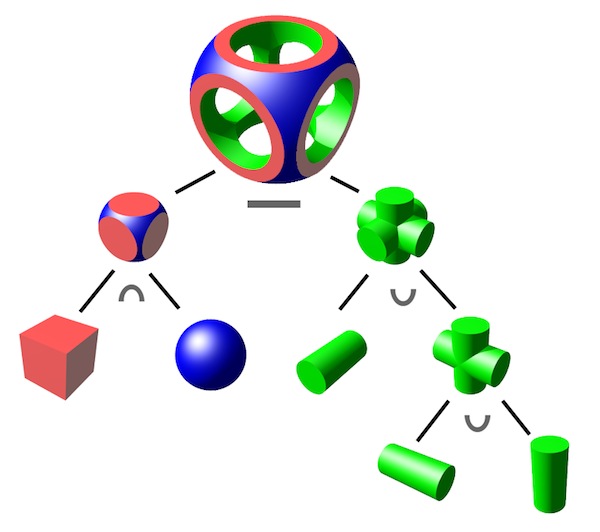
CSG is built on 3 primitive operations: intersection ( $ \cap $ ), union ( $ \cup $ ), and difference ( $ - $ ).

It turns out these operations are all concisely expressible when combining two surfaces expressed as SDFs.

float intersectSDF(float distA, float distB) {
    return max(distA, distB);
}

float unionSDF(float distA, float distB) {
    return min(distA, distB);
}

float differenceSDF(float distA, float distB) {
    return max(distA, -distB);
}

If you set up a scene like this:

float sceneSDF(vec3 samplePoint) {
    float sphereDist = sphereSDF(samplePoint / 1.2) * 1.2;
    float cubeDist = cubeSDF(samplePoint) * 1.2;
    return intersectSDF(cubeDist, sphereDist);
}

Then you get something like this (see section below about scaling to see where the division and multiplication by 1.2 comes from).

In this same Shadertoy, you can play around with the union and difference operations too if you edit the code.

It’s interesting to consider the SDF produced by these binary operations to try to build an intuition for why they work.

$$ \begin{aligned} sceneSDF(\vec p) &= intersectSDF(cube(\vec p), sphere(\vec p)) \\ &= max(cube(\vec p), sphere(\vec p)) \end{aligned} $$

Remember that the region where an SDF is negative represents the interior of the surface. For the above intersection, the $ sceneSDF $ can only be negative if both $ cube(\vec p) $ and $ sphere(\vec p) $ are negative. Which means that we only consider a point inside the scene surface if it’s inside both the cube and the sphere. Which is exactly the definition of CSG intersection!

The same kind of logic applies to union. If either function is negative, the resulting scene SDF will be negative, and therefore inside the surface.

$$ \begin{aligned} sceneSDF(\vec p) &= unionSDF(cube(\vec p), sphere(\vec p)) \\ &= min(cube(\vec p), sphere(\vec p)) \end{aligned} $$

The difference operation was the trickiest for me to wrap my head around.

$$ \begin{aligned} sceneSDF(\vec p) &= differenceSDF(cube(\vec p), sphere(\vec p)) \\ &= max(cube(\vec p), -sphere(\vec p)) \end{aligned} $$

What does the negation of an SDF mean?

If you think again about what the negative and positive region of the SDF mean, you can see that the negative of an SDF is an inversion of the inside and outside of a surface. Everything that was considered inside the surface is now considered outside and vice versa.

This means you can consider the difference to be the intersection of the first SDF and the inversion of the second SDF. So the resulting scene SDF is only negative when the first SDF is negative and the second SDF is positive.

Switching back to geometric terms, that means that we’re inside the scene surface if and only if we’re inside the first surface and outside the second surface – exactly the definition of CSG difference!

Model Transformations

Being able to move the camera gives us some flexibility, but being able to move individual parts of the scene independently of one another certainly gives a lot more. Let’s explore how to do that.

Rotation and Translation

To translate or rotate a surface modeled as an SDF, you can apply the inverse transformation to the point before evaluating the SDF.

Just as you can apply different transformations to different meshes, you can apply different transformations to different parts of the SDF – just only send the transformed ray to the part of the SDF you’re interested in. For instance, to make the cube bob up and down, leaving the sphere in place, but still taking the intersection, you can do this:

float sceneSDF(vec3 samplePoint) {
    float sphereDist = sphereSDF(samplePoint / 1.2) * 1.2;
    float cubeDist = cubeSDF(samplePoint + vec3(0.0, sin(iGlobalTime), 0.0));
    return intersectSDF(cubeDist, sphereDist);
}

Shadertoy reference note: iGlobalTime is a uniform variable set by Shadertoy that contains the number of seconds since playback started.

If you do transformations like this, is the resulting function still a signed distance field? For rotation and translation, it is, because they are “rigid body transformations”, meaning they preserve the distances between points.

More generally, you can apply any rigid body transformation by multiplying the sampled point by the inverse of your transformation matrix.

For instance, if I wanted to apply a rotation matrix, I could do this:

mat4 rotateY(float theta) {
    float c = cos(theta);
    float s = sin(theta);

    return mat4(
        vec4(c, 0, s, 0),
        vec4(0, 1, 0, 0),
        vec4(-s, 0, c, 0),
        vec4(0, 0, 0, 1)
    );
}

float sceneSDF(vec3 samplePoint) {
    float sphereDist = sphereSDF(samplePoint / 1.2) * 1.2;

    vec3 cubePoint = (invert(rotateY(iGlobalTime)) * vec4(samplePoint, 1.0)).xyz;

    float cubeDist = cubeSDF(cubePoint);
    return intersectSDF(cubeDist, sphereDist);
}

…but if you’re using WebGL here, there’s no built in matrix inversion routine in GLSL for now, but you can just do the opposite transform. So the above scene function changes to the equivalent:

float sceneSDF(vec3 samplePoint) {
    float sphereDist = sphereSDF(samplePoint / 1.2) * 1.2;

    vec3 cubePoint = (rotateY(-iGlobalTime) * vec4(samplePoint, 1.0)).xyz;

    float cubeDist = cubeSDF(cubePoint);
    return intersectSDF(cubeDist, sphereDist);
}

For more transformation matrices, refer to any intro to graphics textbook, or check out these slides: 3D Affine transforms.

Uniform Scaling

Okay, let’s get back to this weird scaling trick we glossed over before:

float sphereDist = sphereSDF(samplePoint / 1.2) * 1.2;

The division by 1.2 is scaling the sphere up by 1.2x (remember that we apply the inverse transform to the point before sending it to the SDF). But why do we multiply by the scaling factor afterwards? Let’s examine doubling the size for the sake of simplicity.

float sphereDist = sphereSDF(samplePoint / 2) * 2;

Scaling is not a rigid body transformation – it doesn’t preserve the distance between points. If we transform $ (0, 0, 1) $ and $ (0, 0, 2) $ by dividing them by 2 (which results in a uniform upscaling of the model), then the distance between the points switches from 1 to 0.5.

$$ \begin{aligned} ||(0, 0, 1) - (0, 0, 2)|| &= 1 \\ ||(0, 0, 1) - (0, 0, 0.5)|| &= 0.5 \end{aligned} $$

So when we sample our scaled point in sphereSDF, we’d end up getting back half the distance that the point really is from the surface of our transformed sphere. The multiplication at the end is to compensate for this distortion.

Interestingly, if we try this out in a shader, and use no scale correction, or a smaller value for scale correction, the exact same thing is rendered. Why?

// All of the following result in an equivalent image
float sphereDist = sphereSDF(samplePoint / 2) * 2;
float sphereDist = sphereSDF(samplePoint / 2);
float sphereDist = sphereSDF(samplePoint / 2) * 0.5;

Notice that regardless of how we scale the SDF, the sign of the distance returned stays the same. The sign part of “signed distance field” is still working, but the distance part is now lying.

To see why this is a problem, we need to re-examine how the ray marching algorithm works.

Recall that at every step of the ray marching algorithm, we want to move a distance along the view ray equal to the shortest distance to the surface. We predict that shortest distance using the SDF. For the algorithm to be fast, we want the those steps to be as large as possible, but if we undershoot, the algorithm still works, it just requires more iterations.

But if we overestimate distance, we have a real problem. If we try to scale down the model without correction, like this:

float sphereDist = sphereSDF(samplePoint / 0.5);

Then the sphere disappears completely. If we overestimate the distance, our raymarching algorithm might step past the surface, never finding it.

For any SDF, we can safely scale it uniformly like so:

float dist = someSDF(samplePoint / scalingFactor) * scalingFactor;

Non-uniform scaling and beyond

If we want to scale a model non-uniformly, how can we safely avoid the distance overestimation problem described in the scaling section above? Unlike in uniform scaling, we can’t exactly compensate for the distance distortion caused by the transform. It was possible in uniform scaling because all dimensions were scaled equally, so regardless of where the closest point on the surface to the sampling point is, the scaling compensation will be the same.

But for non-uniform scaling, we need to know where the closest point on the surface is to know how much to correct the distance by.

To see why this is the case, consider the SDF for the unit sphere, scaled to half its size along the x axis, with its other dimensions preserved.

$$ \begin{aligned} sphereSDF(x, y, z) &= \sqrt{(2x)^2 + y^2 + z^2} - 1 \\ \end{aligned} $$

If we evaluate the SDF at $ (0, 2, 0) $, we get back a distance of 1 unit. This is correct: the closest point on the surface of the sphere is $ (0, 1, 0) $. But if evaluate at $ (2, 0, 0) $, we get back a distance of 3 units, which is not right. The closest point on the surface is $ (0.5, 0, 0) $, yielding a world-coordinate distance of 1.5 units.

So, just as in uniform scaling, we need to correct the distance returned by the SDF to avoid overestimating the distance, but by how much? The overestimation factor varies depending on where the point is and where the surface is.

Since it’s usually okay to underestimate the distance, we can just multiply by the smallest scaling factor, like so:

float dist = someSDF(samplePoint / vec3(s_x, s_y, s_z)) * min(s_x, min(s_y, s_z));

The principle for other non-rigid transformations is the same: as long as the sign is preserved by the transformation, you just need to figure out some compensation factor to ensure that you’re never overestimating the distance to the surface.

Putting it all together

With the primitives in this post, you can now create some pretty interesting, complex scenes. Combining those with a simple trick of using the normal vector as the ambient/diffuse component of the material, and you can create something like the shader at the start of the post. Here it is again.

References

There is way more to learn about rendering signed distance functions. One of the most profilic writers on the subject is Inigo Quilez. I learned most of the content of this post from reading his website and his shader code. He’s also one of the co-creators of Shadertoy.

Some of the interesting SDF related material from his site that I didn’t cover at all includes smooth blending between surfaces and soft shadows.

Other references: