Simulating the Physical World

Move your mouse left and right to control the wind.

This post is also available in Russian: Симуляция физического мира.

How might you go about simulating rain? Or any physical process over time, for that matter?

In a simulation, whether it be rain, the airflow over a plane wing, or a slinky slinking down some stairs, we can frame the entire simulation with two pieces of information:

What is the state of everything at the beginning of the simulation?
How does that state change from one moment of time to the next?

By “state of everything”, I mean any non-constant information needed either to determine what the scene looks like at a given moment, or about how the scene will change from one moment to the next. The position of a raindrop, the direction of the wind, and the velocity of each piece of the slinky are all examples of state.

If we represent the entire state of our scene with one big vector $ \vec y $, then we can mathematically reformulate the two pieces of information above into these two statements:

What is a value $y_0$ that satisfies $ y(t_0) = y_0 $?
What is a function $f $ that satisfies $ \frac{dy(t)}{dt} = f(t, y(t)) $?

If you’re confused about why you’d want to store the whole state in one big vector, bear with me. This is one of those cases where it might seem we go way over the top with generality, but I promise there are some interesting tidbits from looking at a general model for simulation.

If you’re confused about how you might store the whole state of a scene in one big vector, let’s look at a simple example. Let’s consider a 2D simulation with 2 particles. Each particle has a position $ \vec x $ and a velocity $ \vec v $.

So to make $ \vec y $, all we have to do is smoosh $ \vec x_1 $, $ \vec v_1 $, $ \vec x_2 $, and $ \vec v_2 $ into one 8 element vector, like this:

$$ \vec y = \begin{bmatrix} \vec x_1 \\ \vec v_1 \\ \vec x_2 \\ \vec v_2 \end{bmatrix} = \begin{bmatrix} x_{1x} \\ x_{1y} \\ v_{1x} \\ v_{1y} \\ x_{2x} \\ x_{2y} \\ v_{2x} \\ v_{2y} \end{bmatrix} $$

And if you’re confused why we want to find $ f(t, y(t)) $ instead of any old definition of $ \frac{dy(t)}{dt} $, the point is to find the derivative only terms of our current state, $ y(t) $, constants, and the time itself. If that’s impossible, it likely that there’s some bit of state we forgot to consider.

The Initial State

Defining $ \vec y_0 $ defines the initial state of the simulation. So if the initial state of our two-particle simulation looks something like this:

Then our numerical initial conditions might look like this:

$$ \vec x_1(t_0) = \begin{bmatrix} 2 \\ 3 \end{bmatrix}, \vec v_1(t_0) = \begin{bmatrix} 1 \\ 0 \end{bmatrix}, \vec x_2(t_0) = \begin{bmatrix} 4 \\ 1 \end{bmatrix}, \vec v_2(t_0) = \begin{bmatrix} -1 \\ 0 \end{bmatrix} $$

Smooshing that together into a single vector, we get our $ \vec y_0 $.

$$ \vec y_0 = \vec y(t_0) = \begin{bmatrix} x_{1x} \\ x_{1y} \\ v_{1x} \\ v_{1y} \\ x_{2x} \\ x_{2y} \\ v_{2x} \\ v_{2y} \end{bmatrix} = \begin{bmatrix} 2 \\ 3 \\ 1 \\ 0 \\ 4 \\ 1 \\ -1 \\ 0 \end{bmatrix} $$

The Derivative Function

$ \vec y_0 $ tells us the initial state, so now all we need is some way of getting from the initial state to the state a tiny bit into the future, and from that state a tiny bit further, and so on.

With that in mind, let’s solve for $ f $ in the equation $ \frac{dy(t)}{dt} = f(t, y(t)) $. So let’s take the derivative of $ y(t) $.

$$ \frac{dy(t)}{dt} = \frac{d}{dt} \begin{bmatrix} x_{1x} \\ x_{1y} \\ v_{1x} \\ v_{1y} \\ x_{2x} \\ x_{2y} \\ v_{2x} \\ v_{2y} \end{bmatrix} = \begin{bmatrix} \frac{dx_{1x}}{dt} \\ \\ \frac{dx_{1y}}{dt} \\ \\ \frac{dv_{1x}}{dt} \\ \\ \frac{dv_{1y}}{dt} \\ \\ \frac{dx_{2x}}{dt} \\ \\ \frac{dx_{2y}}{dt} \\ \\ \frac{dv_{2x}}{dt} \\ \\ \frac{dv_{2y}}{dt} \end{bmatrix} $$

Woah! That’s a tall formula! Don’t worry, we can hopefully make it feel less intimidating by breaking $ \vec y $ back out to its constituent parts.

$$\begin{aligned} \frac{d \vec x_1(t)}{dt} = \begin{bmatrix} \frac{dx_{1x}}{dt} \\ \\ \frac{dx_{1y}}{dt} \end{bmatrix}, \frac{d \vec v_1(t)}{dt} = \begin{bmatrix} \frac{dv_{1x}}{dt} \\ \\ \frac{dv_{1y}}{dt} \end{bmatrix} \\ \\ \frac{d \vec x_2(t)}{dt} = \begin{bmatrix} \frac{dx_{2x}}{dt} \\ \\ \frac{dx_{2y}}{dt} \end{bmatrix}, \frac{d \vec v_2(t)}{dt} = \begin{bmatrix} \frac{dv_{2x}}{dt} \\ \\ \frac{dv_{2y}}{dt} \end{bmatrix} \end{aligned}$$

$ \vec x_1 $ and $ \vec x_2 $ are going to follow similar rules to one another, as will $ \vec v_1 $ and $ \vec v_2 $. So despite the ball of notation above, all we really want to find are the following two things:

$$ \frac{d \vec x}{dt} \textnormal{ and } \frac{d \vec v}{dt} $$

How we define those two derivatives is the real nuts and bolts of the simulation, and to make this an interesting simulation and not just a program where random stuff happens, we can to look to physics for inspiration.

Kinematics & Dynamics

A bit of introductory kinematics and dynamics will go a long way in making our simulation interesting. Let’s start with the real basics.

$ \vec x $ represents position, and the first derivative of position with respect to time is velocity, $ \vec v $. In turn, the first derivative of velocity with respect to time is acceleration, $ \vec a $.

It might seem by now that we’ve already answered our question of finding our derivative function $ f $, since we know the following:

$$ \frac{d \vec x}{dt} = \vec v \textnormal{ and } \frac{d \vec v}{dt} = \vec a $$

We have indeed rather nailed down $ \frac{d \vec x}{dt} $ since $ \vec v $ is part of our state vector $ \vec y(t) $, but we’ll need to go a teensy bit further for the second equation since $ \vec a $ is not.

Newton’s second law comes in handy here: $ \vec F = m \vec a $. If we assume the mass of our particles are known, then we can re-arrange that equation and we’re left with this:

$$ \frac{d \vec v}{dt} = \vec a = \frac{\vec F}{m} $$

Well hold on, $ \vec a $ wasn’t part of $ \vec y(t) $, neither is $ \vec F $, so this hardly seems like progress (remember, we need our derivative function to only be a function of $ \vec y(t) $ and $ t $). But indeed it is progress, because we have all sorts of handy formulas that govern forces in the natural world.

Let’s pretend, for our simple example, that the only force acting upon the particles is the gravitational attraction between them. In that case, we can determine $ \vec F $ using Newton’s law of universal gravitation:

$$ F = G \frac{m_1 m_2}{r^2} $$

Where $ G $ is the gravitational constant $ 6.67 \times 10^{-11} \frac{Nm^2}{kg^2} $, and $ m_1 $ and $ m_2 $ are the masses of our particles (which we assume are constant).

In order to do our simulation, we need a direction too, and we also need to define $ r $ in terms of some part of $ \vec y(t) $. If we say that $ \vec F_1 $ is the force acting upon particle 1, then we can do that like so:

$$\begin{aligned} \vec F_1 &= G \frac{m_1 m_2}{|\vec x_2 - \vec x_1|^2} \left[ \frac{\vec x_2 - \vec x_1}{|\vec x_2 - \vec x_1|} \right] = G \frac{m_1 m_2(\vec x_2 - \vec x_1)}{|\vec x_2 - \vec x_1|^3} \\ \\ \vec F_2 &= G \frac{m_2 m_1}{|\vec x_1 - \vec x_2|^2} \left[ \frac{\vec x_1 - \vec x_2}{|\vec x_1 - \vec x_2|} \right] = G \frac{m_2 m_1(\vec x_1 - \vec x_2)}{|\vec x_1 - \vec x_2|^3} \end{aligned}$$

Let’s recap. The changing state of our two particle system is entirely described by $ \vec x_1, $ $ \vec v_1, $ $ \vec x_2, $ and $ \vec v_2 $. And those change over time like so:

$$\begin{aligned} \frac{d \vec x_1}{dt} &= \vec v_1 \\ \\ \frac{d \vec x_2}{dt} &= \vec v_2 \\ \\ \frac{d \vec v_1}{dt} &= \vec a_1 = \frac{\vec F_1}{m_1} = G \frac{m_2 (\vec x_2 - \vec x_1)}{|\vec x_2 - \vec x_1|^3} \\ \\ \frac{d \vec v_2}{dt} &= \vec a_2 = \frac{\vec F_2}{m_2} = G \frac{m_1 (\vec x_1 - \vec x_2)}{|\vec x_1 - \vec x_2|^3} \end{aligned}$$

Now we have all the information that makes this simulation different from all other simulations: $\vec y_0$ and $f$.

$$\begin{aligned} \vec y_0 &= \vec y(0) &= \begin{bmatrix} \vec x_1(0) \\ \vec v_1(0) \\ \vec x_2(0) \\ \vec v_2(0) \end{bmatrix} &= \begin{bmatrix} (2, 3) \\ (1, 0) \\ (4, 1) \\ (-1, 0) \end{bmatrix} \\ \\ f(t, y(t)) &= \frac{d\vec y}{dt}(t) &= \begin{bmatrix} \frac{d\vec x_1}{dt}(t) \\ \\ \frac{d\vec v_1}{dt}(t) \\ \\ \frac{d\vec x_2}{dt}(t) \\ \\ \frac{d\vec v_2}{dt}(t) \end{bmatrix} &= \begin{bmatrix} \vec v_1(t) \\ \\ G \frac{m_2 \big(\vec x_2(t) - \vec x_1(t)\big)}{|\vec x_2(t) - \vec x_1(t)|^3} \\ \\ \vec v_2(t) \\ \\ G \frac{m_1 \big(\vec x_1(t) - \vec x_2(t)\big)}{|\vec x_1(t) - \vec x_2(t)|^3} \end{bmatrix} \end{aligned}$$

Now then, now that we have a rigorously defined simulation, how might we go about turning it into a mesmerizing animation?

In case you’ve written simulations or games before, you might jump to something like this:

x += v * delta_t
v += F/m * delta_t

Let’s take a step back and consider why that works.

A Differential Equation

Before diving into implementation, let’s step back a second and see what information we have and what information we need. We have a $ y_0 $ that satisfies $ y(t_0) = y_0 $, and we have an $ f $ that satisfies $ \frac{dy}{dt}(t) = f(t, y(t)) $. What we want is a function that can predict the state of the system at any point in time. Phrased mathematically, we want $ y(t) $.

With this in mind, if you squint carefully at $ \frac{dy}{dt}(t) = f(t, y(t)) $, you might spy that it’s an equation that relates $ y $ with its derivative $ \frac{dy}{dt} $. That makes it a differential equation! More specifically, it makes it a first order, ordinary differential equation. If we solve this differential equation, we get the function $ y(t) $.

Solving for $ y(t) $ given $ y_0 $ and $ f $ is called an initial value problem.

Numerical Integration

Some initial value problems have easily found analytic solutions, but for complex simulations this tends to be infeasible. So let’s try to figure out a method of approximating the solution.

Let’s explore a simpler initial value problem:

Given $ y(0) = 1 $ and $ \frac{dy}{dt}(t) = f(t, y(t)) = y(t) $, find an approximation of $ y(t) $.

Let’s examine the problem from a graphical perspective by considering the value and tangent line at $t = 0 $. From our givens, we have $ y(0) = 1 $ and $ \frac{dy}{dt}(t) = y(t) = 1 $.

So we don’t know what $ y(t) $ looks like yet, but we do know that it should follow the tangent line near to $ t = 0 $. So let’s estimate $ y(0 + h) $ for some small value of $ h $ by following the tangent line. We’ll use $ h = 0.5 $ for now.

Symbolically, we’re estimating $ y(h) $ like so:

$$\begin{aligned} y(h) \approx y(0) + h \frac{dy}{dt}(0) &= y(0) + h f(0, y(0)) \\ &= y(0) + h y(0) \\ &= 1 + h \end{aligned}$$

So for $ h = 0.5 $, $ y(h) \approx 1.5 $.

Now we can repeat this process. Even though we don’t know the exact value of $ y(h) $, as long as we have a pretty good approximation of it, we can figure out a pretty good approximation of the tangent line at that point too!

$$\begin{aligned} f(t, y(t)) &= y(t) \\ f(0.5, 1.5) &= 1.5 \end{aligned}$$

Then we can follow this tangent line $ h $ units to the right as well.

We can repeat the process again, with a tangent slope of $ f(t, y(t)) = f(1, 2.25) = 2.25$:

Stating the procedure recursively, we have this:

$$\begin{aligned} t_{i+1} &= t_i + h \\ y_{i+1} &= y_i + h f(t_i, y_i) \end{aligned}$$

This is called the “Forward Euler” method of numerical integration. This is the general case of the step x += v * delta_t!

In this particular initial value problem, our steps look like so:

$$\begin{aligned} t_{i+1} &= t_i + h \\ y_{i+1} &= y_i + h y_i \end{aligned}$$

This method lends itself well to representing the computations in a table, like so:

$$\begin{aligned} t_0 &= 0, & y_0 &= 1 & & &\\ t_1 &= 0.5, & y_1 &= y_0 + h y_0 &=& 1 + 0.5 (1) &=& 1.5 \\ t_2 &= 1, & y_2 &= y_1 + h y_1 &=& 1.5 + 0.5 (1.5) &=& 2.25 \\ t_3 &= 1.5, & y_3 &= y_2 + h y_2 &=& 2.25 + 0.5 (2.25) &=& 3.375 \\ \end{aligned}$$

It turns out that this particular initial value problem has a nice analytical solution: $ y(t) = e^t $

Graph of $ y(t) = e^t $

When approximating the solution with Forward Euler, what do you think happens as the time step $ h $ gets smaller?

$ h=0.5 $

Move the slider left and right to control the value of h.

The error between the approximate solution and the exact solution decreases as $ h $ decreases! In addition to decreasing $ h $ to decrease the error, you could also use an alternative method of numerical integration that may provide better error bounds, such as the Midpoint method, Runge-Kutta methods, and linear multistep methods.

Let’s get coding!

Just as we can generalize the definition of a simulation mathematically, we can generalize the implementation of a simulation programmatically.

Since I’m most familiar with JavaScript but appreciate the clarity type annotations can give code, all the code samples will be written in TypeScript.

Let’s start with a version that assumes that y is a one-dimensional array of numbers, just as in the mathematical explorations.

function runSimulation(
    // y(0) = y0
    y0: number[],
    // dy/dt(t) = f(t, y(t))
    f: (t: number, y: number[]) => number[],
    // display the current state of the simulation
    render: (y: number[]) => void
) {
    // Step forward 1/60th of a second at a time
    // This results in realtime simulation if playback is 60fps
    const h = 1 / 60.0;

    function simulationStep(ti: number, yi: T) {
        render(yi)
        requestAnimationFrame(function() {
            const fi = f(ti, yi)

            // t_{i+1} = t_i + h
            const tNext = ti + h

            // y_{i+1} = y_i + h f(t_i, y_i)
            const yNext = []
            for (let j = 0; j < y.length; j++) {
                yNext.push(yi[j] + h * fi[j]);
            }

            simulationStep(tNext, yNext)
        })
    }
    simulationStep(0, y0)
}

It turns out to be pretty inconvenient to always operate on 1-dimensional arrays of numbers, so we can abstract away the addition and multiplication operations on the simulation state into an interface, then define our general simulation code concisely using TypeScript Generics¹.

interface Numeric<T> {
    plus(other: T): T
    times(scalar: number): T
}

function runSimulation<T extends Numeric<T>>(
  y0: T,
  f: (t: number, y: T) => T,
  render: (y: T) => void
) {
    const h = 1 / 60.0;

    function simulationStep(ti: number, yi: T) {
        render(yi)
        requestAnimationFrame(function() {
            // t_{i+1} = t_i + h
            const tNext = ti + h
            // y_{i+1} = y_i + h f(t_i, y_i)
            const yNext = yi.plus(f(ti, yi).times(h))
            simulationStep(yNext, tNext)
        })
    }
    simulationStep(y0, 0.0)
}

The cool thing about having this general code is it lets us focus on the core of the simulation: what about this simulation is different from other simulations. Using the example of our two particle simulation from before:

// Represents the state of the entire
// two particle simulation at a point in time.
class TwoParticles implements Numeric<TwoParticles> {
    constructor(
        readonly x1: Vec2, readonly v1: Vec2,
        readonly x2: Vec2, readonly v2: Vec2
    ) { }

    plus(other: TwoParticles) {
        return new TwoParticles(
            this.x1.plus(other.x1), this.v1.plus(other.v1),
            this.x2.plus(other.x2), this.v2.plus(other.v2)
        );
    }

    times(scalar: number) {
        return new TwoParticles(
            this.x1.times(scalar), this.v1.times(scalar),
            this.x2.times(scalar), this.v2.times(scalar)
        )
    }
}

// dy/dt (t) = f(t, y(t))
function f(t: number, y: TwoParticles) {
    const { x1, v1, x2, v2 } = y;
    return new TwoParticles(
        // dx1/dt = v1
        v1,
        // dv1/dt = G*m2*(x2-x1)/|x2-x1|^3
        x2.minus(x1).times(G * m2 / Math.pow(x2.minus(x1).length(), 3)),
        // dx2/dt = v2
        v2,
        // dv2/dt = G*m1*(x1-x1)/|x1-x2|^3
        x1.minus(x2).times(G * m1 / Math.pow(x1.minus(x2).length(), 3))
    )
}

// y(0) = y0
const y0 = new TwoParticles(
    /* x1 */ new Vec2(2, 3),
    /* v1 */ new Vec2(1, 0),
    /* x2 */ new Vec2(4, 1),
    /* v2 */ new Vec2(-1, 0)
)

const canvas = document.createElement("canvas")
canvas.width = 400;
canvas.height = 400;
const ctx = canvas.getContext("2d")!;
document.body.appendChild(canvas);

// Display the current state of the simulation
function render(y: TwoParticles) {
    const { x1, x2 } = y;
    ctx.fillStyle = "white";
    ctx.fillRect(0, 0, 400, 400);

    ctx.fillStyle = "black";
    ctx.beginPath();
    ctx.ellipse(x1.x*50 + 200, x1.y*50 + 200, 15, 15, 0, 0, 2 * Math.PI);
    ctx.fill();

    ctx.fillStyle = "red";
    ctx.beginPath();
    ctx.ellipse(x2.x*50 + 200, x2.y*50 + 200, 30, 30, 0, 0, 2 * Math.PI);
    ctx.fill();
}

// Run the thing!
runSimulation(y0, f, render)

If we tweak the numbers a bit, we can get a simulation of the moon’s orbit!

Earth-Moon orbital simulation, 1px=2500km.
1 second of simulation time is 1 day of real-world time.
Earth & Moon are shown at 10x their correct proportional size.

If you want to play with the code, here it is: Earth Moon Simulation on Codepen.

Collisions & Constraints

While that mathematical model of things I presented does model the physical world, the numerical integration method sadly falls apart in certain situations.

Consider a simulation of a bouncing ball.

The entire state of the simulation is:

$$ \vec y = \begin{bmatrix} x \\ v \end{bmatrix} $$

Where $ x $ is the ball’s height off the ground and $ v $ is the velocity of the ball. If we drop the ball from a height of 0.8 meters, we have:

$$ \vec y_0 = \begin{bmatrix} 0.8 \\ 0 \end{bmatrix} $$

If we plot $ x(t) $, it would look something like this:

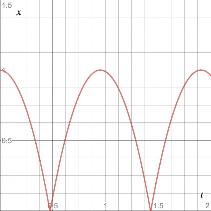
While the ball is falling, we can construct our derivative function $ f $ fairly easily:

$$ f(t, y(t)) = \frac{dy}{dt}(t) = \begin{bmatrix} \frac{dx}{dt}(t) \\ \\ \frac{dv}{dt}(t) \end{bmatrix} = \begin{bmatrix} v \\ a \end{bmatrix} $$

While accelerating only under the influence of gravity, $ a = -g = -9.8 \frac{m}{s^2} $.

But what happens when the ball hits the ground? We know the ball has hit the ground when $ x = 0 $. But in our numerical integration, it’s possible that the ball might be above the ground at one time step, and in the ground the next time step: $ x_i > 0, x_{i+1} < 0 $.

We could solve this by rewinding time to find the time $ t_c $ at which the collision happens $ (t_i < t_c < t_{i+1}) $. But once we’ve found that, we still don’t have a way to define $ \frac{dv}{dt} $ that would result in the velocity instantaneously changing to be upwards instead of downwards.

It’s possible to work this all out by having the collision take a finite amount of time to take place and applying some force $ F $ over that timespan $ \Delta t $, but it’s usually easier to just support some kind of discrete constraints to the simulation.

We can also do more than one iteration of the physics simulation per rendered frame to reduce the amount by which the ball penetrates the floor before bouncing. With that in mind, our core simulation code changes to this:

function runSimulation<T extends Numeric<T>>(
  y0: T,
  f: (t: number, y: T) => T,
  applyConstraints: (y: T) => T,
  iterationsPerFrame: number,
  render: (y: T) => void
) {
    const frameTime = 1 / 60.0
    const h = frameTime / iterationsPerFrame

    function simulationStep(yi: T, ti: number) {
        render(yi)
        requestAnimationFrame(function () {
            for (let i = 0; i < iterationsPerFrame; i++) {
                yi = yi.plus(f(ti, yi).times(h))
                yi = applyConstraints(yi)
                ti = ti + h
            }
            simulationStep(yi, ti)
        })
    }
    simulationStep(y0, 0.0)
}

And then we can implement our bouncing ball like so:

const g = -9.8; // m / s^2
const r = 0.2; // m

class Ball implements Numeric<Ball> {
    constructor(readonly x: number, readonly v: number) { }
    plus(other: Ball) { return new Ball(this.x + other.x, this.v + other.v) }
    times(scalar: number) { return new Ball(this.x * scalar, this.v * scalar) }
}

function f(t: number, y: Ball) {
    const { x, v } = y
    return new Ball(v, g)
}

function applyConstraints(y: Ball): Ball {
    const { x, v } = y
    if (x <= 0 && v < 0) {
        return new Ball(x, -v)
    }
    return y
}

const y0 = new Ball(
    /* x */ 0.8,
    /* v */ 0
)

function render(y: Ball) {
    ctx.clearRect(0, 0, 400, 400)
    ctx.fillStyle = '#EB5757'
    ctx.beginPath()
    ctx.ellipse(200, 400 - ((y.x + r) * 300), r * 300, r * 300, 0, 0, 2 * Math.PI)
    ctx.fill()
}

runSimulation(y0, f, applyConstraints, 30, render)

You can play around with this version of the code here: Bouncing Ball on Codepen.

Implementers beware!

While this general description of simulations has some nice properties, it doesn’t necessarily yield the most high performance simulations. I find it a nice framework to think about the behavior of simulations, though there’s certainly a lot of unnecessary overhead.

The rain simulation that starts this post is, for instance, not implemented using the patterns here. Instead, it was an experiment using the Entity Component System architectural pattern. You can see the source for the rain simulation here: Rain Simulation source on GitHub.

Until next time!

Something about the intersection of math, physics, and programming really strikes a chord with me. Getting simulations up and running and rendering makes for a very special kind of something out of nothing.

SIGGRAPH course notes served as a form of inspiration here, just as they did with the fluid simulation. Check out “An Introduction to Physically Based Modelling” course notes from SIGGRAPH 2001 if you want a much more rigorous look into this material. I have the notes from 1997 linked because it looks like Pixar took the 2001 versions down.

Thanks to Maggie Cai for the beautiful illustration of the couple with the umbrella and for having the patience to meticulously choose colors when I can barely tell the difference between blue and grey.

And in case you were wondering, the illustration was made in Figma. 😃

The same pattern would work using duck typing in dynamic languages like Python and JavaScript. This pattern would be nicer in languages supporting operator overloading, such as Python, C++, Scala, etc. ^[return]